池田写像

物理学や数学において、池田写像 (いけだしゃぞう、英語: Ikeda map) は以下の複素解析写像で与えられる離散時間力学系である。

z_{n+1}=A+Bz_{n}e^{i(|z_{n}|^{2}+C)}

オリジナルの池田写像は非線形光共振器 (リングレーザー（英語版）、非線形誘電体を含む) における光の軌跡のモデルとして池田研介により提案された。池田研介、大同寛明、秋元興一により上記の単純化した形に一般化された^[1]。

$z_{n}$ は共振器内の回転のn番目のステップにおける共振器内の電場を表し、 $A$ と $C$ はそれぞれ、外部からのレーザー光線と共振器の線形位相を示すパラメータである。

特に、パラメータ $B(<=1)$ は振る舞いを特徴づける散逸パラメータと呼ばれ、 $B=1$ の極限で池田写像は保存系になる。

非線形誘電体の飽和効果を考慮に入れ、オリジナルの池田写像に修正を施した以下の形で使用される事が多い。

z_{n+1}=A+Bz_{n}e^{iK/(|z_{n}|^{2}+1)+C}

上記を実2次元平面に描く場合、

x_{n+1}=1+u(x_{n}\cos t_{n}-y_{n}\sin t_{n}),\,

y_{n+1}=u(x_{n}\sin t_{n}+y_{n}\cos t_{n}),\,

となる。ここで、uはパラメータであり、

t_{n}=0.4-{\frac {6}{1+x_{n}^{2}+y_{n}^{2}}}.

である。幾つかの値のuでは、この系はカオスな振る舞いを示す。

アトラクター

この動画はパラメータ $u$ を0.0から1.0まで0.01ずつ変化させた時の挙動を示している。シミュレーションに使用したステップ数は500、ランダムに選択した始点は20000個である。アトラクターを描くため、それぞれの軌道で20個の点がプロットされている。 $u$ の値が増加するにつれ、アトラクターポイントの分岐は大きくなる。

$u=0.3$	$u=0.5$
$u=0.7$	$u=0.9$

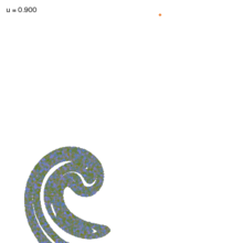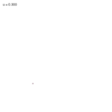
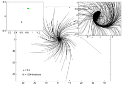
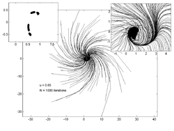
挙動

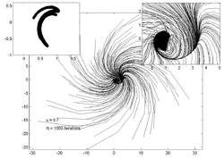
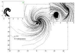
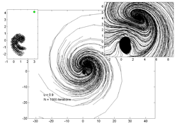
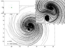
以下の図は、 $u$ の値を変化させた時の200個のランダムな点の動きを表したものである。各々の図の左上にある画像はアトラクターの形成過程を示し、右上の画像は中心部を拡大した画像となっている。

u = 0.1	u = 0.5	u = 0.65
u = 0.7	u = 0.8	u = 0.85
u = 0.9	u = 0.908	u = 0.92

Octave/MATLABコード

このプロットを生成するOctave/MATLABコードを以下に示す。

% u = ikeda parameter
% option = what to plot
%  'trajectory' - plot trajectory of random starting points
%  'limit' - plot the last few iterations of random starting points
function ikeda(u, option)
    P = 200;%how many starting points
    N = 1000;%how many iterations
    Nlimit = 20; %plot these many last points for 'limit' option

    x = randn(1,P)*10;%the random starting points
    y = randn(1,P)*10;

    for n=1:P,
        X = compute_ikeda_trajectory(u, x(n), y(n), N);

        switch option
        case 'trajectory' %plot the trajectories of a bunch of points
            plot_ikeda_trajectory(X);hold on;

        case 'limit'
            plot_limit(X, Nlimit); hold on;

        otherwise
            disp('Not implemented');
        end
    end

    axis tight; axis equal
    text(-25,-15,['u = ' num2str(u)]);
    text(-25,-18,['N = ' num2str(N) ' iterations']);
    end

    % Plot the last n points of the curve - to see end point or limit cycle
    function plot_limit(X,n)
    plot(X(end-n:end,1),X(end-n:end,2),'ko');
end

% Plot the whole trajectory
function plot_ikeda_trajectory(X)
    plot(X(:,1),X(:,2),'k');
    %hold on; plot(X(1,1),X(1,2),'bo','markerfacecolor','g'); hold off
end

%u is the ikeda parameter
%x,y is the starting point
%N is the number of iterations
function [X] = compute_ikeda_trajectory(u, x, y, N)
    X = zeros(N,2);
    X(1,:) = [x y];

    for n = 2:N

        t = 0.4 - 6/(1 + x^2 + y^2);
        x1 = 1 + u*(x*cos(t) - y*sin(t)) ;
        y1 = u*(x*sin(t) + y*cos(t)) ;
        x = x1;
        y = y1;

        X(n,:) = [x y];

    end
end

脚注

^ K.Ikeda, Multiple-valued Stationary State and its Instability of the Transmitted Light by a Ring Cavity System, Opt. Commun. 30 257-261 (1979); K. Ikeda, H. Daido and O. Akimoto, Optical Turbulence: Chaotic Behavior of Transmitted Light from a Ring Cavity, Phys. Rev. Lett. 45, 709–712 (1980)